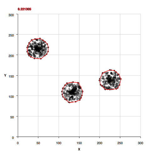
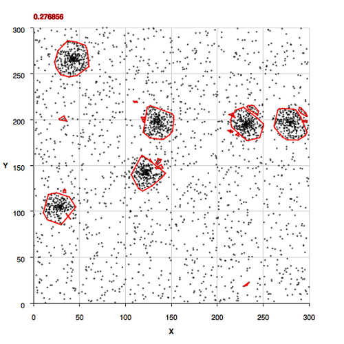
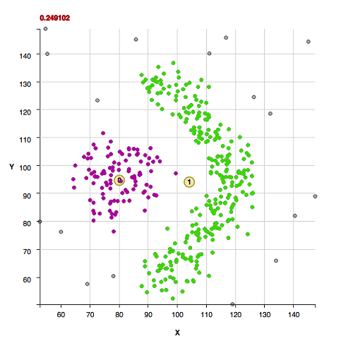
This is the web page for the older, density based algorithm in the project which is based upon distances between voids and fits to a Generalized Extreme Value function. Its runtime complexity is between O(Npoints2) and O(Npoints3) while the newer code presented on the main page has a runtime complexity of O(Npixels X log2(Npixels)).
The code is a density based clustering algorithm. The algorithm does not require prior knowledge of the number of clusters, nor does it require a separation distance for association of points, and the algorithm finds non-convex cluster shapes in a statistically based manner that is reproducable. The algorithm learns the association separation distance of points by the statistics of the data itself and applies that in a critical threshold for membership of points within a cluster.
The algorithm, in an unsupervised manner, constructs histograms of rectangular voids in the data and fits Generalized Extreme Value curves to the histograms to learn the background density. Clusters in the data are found as points that are within a separation distance smaller than the critical density for membership.
The results are available as data and visualized through generated html plots. (Improvements to packaging and documentation are in progress.)
More about the density distribution:
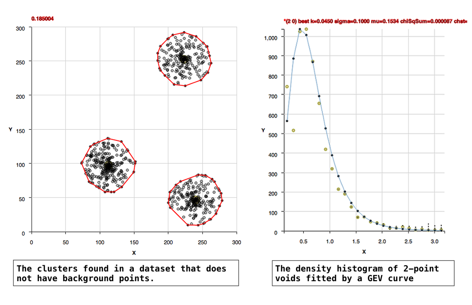
The location of the 'background' points in two dimensional space are likely Poisson, that is their locations in a fixed interval of space are independent of one another and occur randomly. The 2-point void densities are formed into a histogram that is well fit by Generalized Extreme Value (GEV) curves. Extreme value distributions are used to describe the maximum or minimum of values drawn from a sample distribution that is essentially exponential.
There are 2 methods for determining clusters in this code:
(1) For datasets in which there are background points: The peak of the GEV fit should represent the background density. The clusters are then defined statistically as being 2 to 3 times 'above the background', that is having separations 2 to 3 times more dense than the background density. The code by default uses a factor of 2.5, but methods are supplied to allow the user to set the background to 2 or 3 instead, and there's also a method to set the background manually.
The later manual setting is useful for a case where perhaps one determined the background density in one dataset and need to apply that to a 2nd dataset which has the same background, but is 'saturated' with foreground points.(2) For datasets in which there are no background points: Datasets which are only points which should be in groups, and essentially have no background points are referred to as sparse background datasets. For these datasets, the background density is zero, so we define the level above the background by the edges of the densities of the group. This edge density is already much larger than the background so it is the threshold density for membership already. This threshold density is the first x bin in a well formed histogram of 2-point densities.
The code automatically determines which of method (1) and (2) to use.
If the user has better knowledge of which should be applied, can set that with:
useFindMethodForDataWithoutBackgroundPoints()
or useFindMethodForDataWithBackgroundPoints()
The GEV curve contains 3 independent fitting parameters and the curve is an exponential combined with a polynomial, so it's resulting fitted parameters are not unique, but the curve is useful for characterizing the background point distribution by then integrating under the curve.
The points within a cluster are may have interesting distributions that can be better modeled after they've been found by these means.
Usage as an API:
To use the code with default settings:
  TwoPointCorrelation clusterFinder
       = new TwoPointCorrelation(x, y, xErrors, yErrors, totalNumberOfPoints);

  clusterFinder.calculateBackground();

  clusterFinder.findClusters();
The results are available as group points or as convex hulls surrounding the groups:
 int n = clusterFinder.getNumberOfGroups()

 int groupNumber = 0;

 To get the hull for groupId 0:
     ArrayPair hull0 = clusterFinder.getGroupHull(groupNumber);

 To get the points in groupId 0:
     ArrayPair group0 = clusterFinder.getGroup(groupNumber)

 To plot the results:
     String plotFilePath = clusterFinder.plotClusters();
If debugging is turned on, plots are generated and those file paths are printed to standard out, and statements are printed to standard out.
To set the background density manually:
 TwoPointCorrelation clusterFinder
     = new TwoPointCorrelation(x, y, xErrors, yErrors, >getTotalNumberOfPoints());
 clusterFinder.setBackground(0.03f, 0.003f);
 clusterFinder.findClusters();
 String plotFilePath = clusterFinder.plotClusters();
If the centers of the cluster hulls are needed for something else, seeds for a Voronoi diagram, for instance, one can use:
ArrayPair seeds = clusterFinder.getHullCentroids();
The scatter plots and histograms below use d3 js
Note that improvements in the histogram code is *in progress. Currently datasets with a small number of points may have less than ideal solutions.*
Note also that the code has the ability to refine a solution: that is to determine groups and then subtract them from the data and then re-determine the background density from the remaining points. The ability is not enabled by default, but can be with the method setAllowRefinement(). More information is here.
The citation for use of this code in a publication is:
http://code.google.com/p/two-point-correlation/, Nichole King, "Unsupervised Clustering Based Upon Voids in Two-Point Correlation". March 15, 2013.
Note that I wrote the core algorithm in this work (without the automated density calculation) several years ago and the results were part of a publication. What got published was the results from this algorithm used as input for another algorithm that requires knowledge of association radius in order to work. The algorithm that used my algorithm's input required a parameter that was not derivable from it's use alone. Similarly, "k-means clustering" requires knowledge of the number of clusters before use. "k-means++" is an algorithm that suggests one can adjust the number of clusters k, but a statistical method of doing so would still require a density based analysis, and hence, it would need to do the same work as the algorithm here, but presumably less efficiently. Delaunay Triangulation is useful if there are no background points within a dataset, that is all points will be members of a group, and if groups do not have non-convex shapes. KDTrees are useful as a nearest neighbor algorithm, but its use in determining clusters would still require as input, an association radius. Fun stuff, but the core of the algorithm here is was what I needed to create awhile back for work applied to surveys. The addition published here is automation of the background determination and large improvements of the overall algorithm.
Sparsely Populated Background
Moderately Populated Background
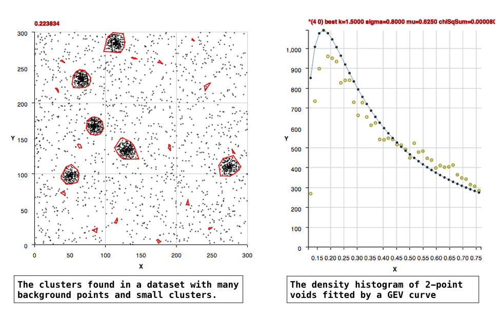
More Densely Populated Background
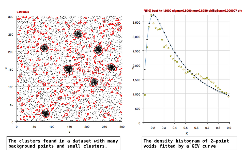
All Background, No Clusters

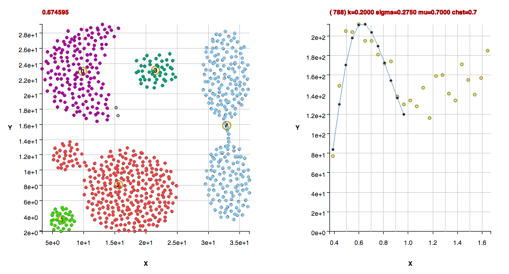
Non-Convex Morphology Clusters

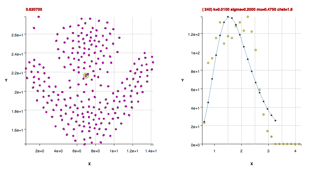
The cluster "shape" datasets collected at http://cs.joensuu.fi/sipu/datasets/ are fit here with explanations of code settings used and comments about the data.
These clusters were found with the default algorithm settings. No additional settings were needed for the background:
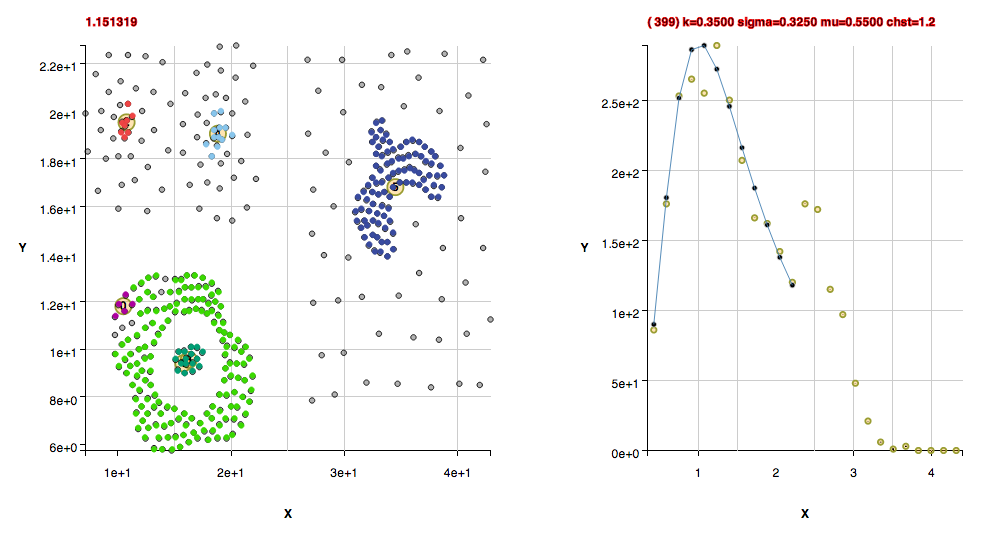
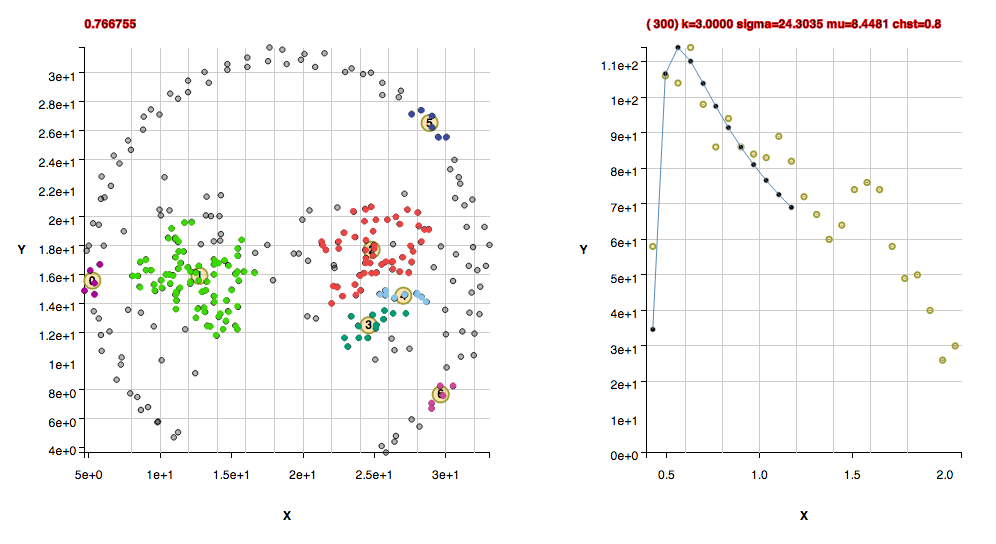
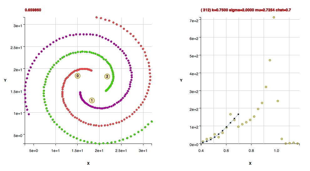

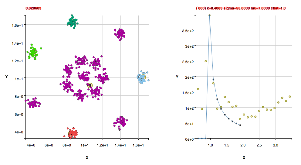
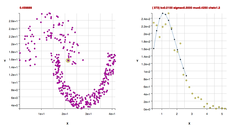
These clusters were found with the default algorithm settings plus using the method useFindMethodForDataWithoutBackgroundPoints();
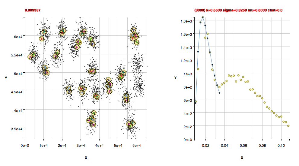
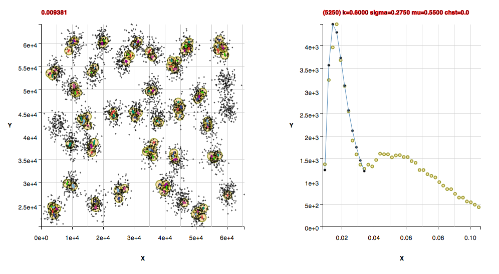
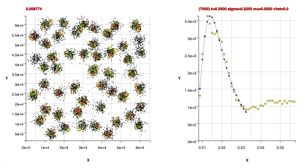
These clusters were found with the default algorithm settings plus using the method useFindMethodForDataWithoutBackgroundPoints(); Note that these next 3 datasets have the uncommon property of being composed of isolated pairs of points, that is, there are never 3 or more points within the pair point separation of one another. If one wanted to apply a slightly agglomerative approach to finding clusters in those datasets, one could use the found cluster centers in a new histogram and determine the critical density from those. That isn't done in this algorithm in order to keep a uniform way of determining clusters in a statistically reproducable manner.
Performance Metrics
Roughly determined by estimation and measured with a very small number of iterations on a computer with characteristics: 64-bit Intel Core 2 Duo processor w/ speed 2 GHz w/ 4 MB L2 Cache 3GB RAM and a bus speed of 800 MHz
JVM characteristics: J2SE 1.6, 64-bit HotSpot server w/ initial heap size 512 MB and max heap size 1024 MB.
Measurements are from the June 29, 2014 code (e35ea01990b54cc8e88b76e9ce30220a35cdb79d).
Runtime (RT) complexity for findVoids() is less than O(N^2) but it invokes functions that vary from O(1) to O(N-1) as it compares the range between points, so best is less than O(N^2) and worse is less than O(N^3). RT complexity for findGroups() is a little worse than O(N^2). The RT complexity for findGroups is a DFS search over sorted x so is < O(N^2) due to being able to truncate the search over potential neighbors.
(NOTE that improvements in findGroups is in progress. The total RT should be smaller afterwards by using memoization w/ Fibonacci Heaps in the findVoids stage to limit the neighbor search in findGroups's DFS.)
Empirically derived runtimes follow.
  N          findVoids        findGroups     Sys load  Total RT
points      RT      mem       RT      mem     at start
         in sec   in MB     in sec  in MB               in sec

   99      0       0.2        0      0.2      0.7        0

 1089      1       20         0      20       0.7        1

 10605     4                  1                          5

101400    29       14        226     21       1          255
Note that for the datasets with number of points > 15000, the void density is determined through partial sampling rather than complete sampling, so there may be a need occasionally to override the automatic decision for sampling in the code. Methods are provided to override defaults.